consistent hashing ���法早在 1997 �q�就在论�?/span> Consistent hashing and random trees 中被提出�Q�目前在 cache �pȝ��中应用越来越�q�泛�Q?/span>
1 基本场景
比如你有 N �?/span> cache 服务器(后面����U?/span> cache �Q�,那么如何���一个对�?/span> object 映射�?/span> N �?/span> cache 上呢�Q�你很可能会采用�c�M��下面的通用�Ҏ��计算 object �?/span> hash ��|��然后均匀的映���到�?/span> N �?/span> cache �Q?/span>
hash(object)%N
一切都�q�行正常�Q�再考虑如下的两�U�情况;
1 一�?/span> cache 服务�?/span> m down 掉了�Q�在实际应用中必��要考虑�q�种情况�Q�,�q�样所有映���到 cache m 的对象都会失效,怎么办,需要把 cache m �?/span> cache 中移除,�q�时�?/span> cache �?/span> N-1 収ͼ�映射公式变成�?/span> hash(object)%(N-1) �Q?/span>
2 �׃��讉K��加重�Q�需要添�?/span> cache �Q�这时�?/span> cache �?/span> N+1 収ͼ�映射公式变成�?/span> hash(object)%(N+1) �Q?/span>
1 �?/span> 2 意味着什么?�q�意味着�H�然之间几乎所有的 cache 都失效了。对于服务器而言�Q�这是一场灾难,�z�水般的讉K��都会直接冲向后台服务器;
再来考虑�W�三个问题,�׃������g能力���来���强�Q�你可能惌���后面��d��的节点多做点�z�,昄���上面�?/span> hash ���法也做不到�?/span>
有什么方法可以改变这个状况呢�Q�这���是 consistent hashing...
2 hash ���法和单调�?/h2>
Hash ���法的一个衡量指标是单调性( Monotonicity �Q�,定义如下�Q?/span>
单调性是指如果已�l�有一些内定w��过哈希分派��C��相应的缓冲中�Q�又有新的缓冲加入到�pȝ��中。哈希的�l�果应能够保证原有已分配的内容可以被映射到新的缓冲中去,而不会被映射到旧的缓冲集合中的其他缓冲区�?/span>
�Ҏ��看到�Q�上面的����?/span> hash ���法 hash(object)%N 难以满��单调性要求�?/span>
3 consistent hashing ���法的原�?/h2>
consistent hashing 是一�U?/span> hash ���法�Q�简单的��_��在移�?/span> / ��d��一�?/span> cache �Ӟ��它能够尽可能���的改变已存�?/span> key 映射关系�Q�尽可能的满���_��调性的要求�?/span>
下面���来按照 5 个步骤简单讲�?/span> consistent hashing ���法的基本原理�?/span>
3.1 环�Şhash �I�间
考虑通常�?/span> hash ���法都是��?/span> value 映射��C���?/span> 32 为的 key ��|��也即�?/span> 0~2^32-1 �ơ方的数值空��_��我们可以���这个空间想象成一个首�Q?/span> 0 �Q�尾�Q?/span> 2^32-1 �Q�相接的圆环�Q�如下面�?/span> 1 所�C�的那样�?/span>
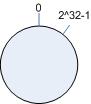
�?/span> 1 环�Ş hash �I�间
3.2 把对象映���到hash �I�间
接下来考虑 4 个对�?/span> object1~object4 �Q�通过 hash 函数计算出的 hash �?/span> key 在环上的分布如图 2 所�C��?/span>
hash(object1) = key1;
… …
hash(object4) = key4;
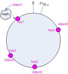
�?/span> 2 4 个对象的 key 值分�?/span>
3.3 把cache 映射到hash �I�间
Consistent hashing 的基本思想���是���对象和 cache 都映���到同一�?/span> hash 数值空间中�Q��ƈ且��用相同的hash ���法�?/span>
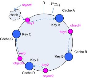
假设当前�?/span> A,B �?/span> C �?/span> 3 �?/span> cache �Q�那么其映射�l�果���如�?/span> 3 所�C�,他们�?/span> hash �I�间中,以对应的 hash值排列�?/span>
hash(cache A) = key A;
… …
hash(cache C) = key C;
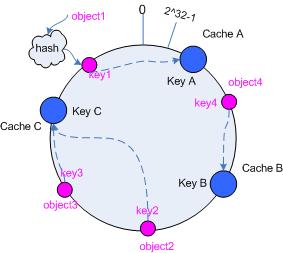
�?/span> 3 cache 和对象的 key 值分�?/span>
说到�q�里�Q�顺便提一�?/span> cache �?/span> hash 计算�Q�一般的�Ҏ��可以使用 cache 机器�?/span> IP 地址或者机器名作�ؓhash 输入�?/span>
3.4 把对象映���到cache
现在 cache 和对象都已经通过同一�?/span> hash ���法映射�?/span> hash 数值空间中了,接下来要考虑的就是如何将对象映射�?/span> cache 上面了�?/span>
在这个环形空间中�Q�如果沿着��时针方向从对象�?/span> key 值出发,直到遇见一�?/span> cache �Q�那么就���该对象存储在这�?/span> cache 上,因�ؓ对象�?/span> cache �?/span> hash 值是固定的,因此�q�个 cache 必然是唯一和确定的。这样不���找��C��对象�?/span> cache 的映���方法了吗?�Q?/span>
依然�l�箋上面的例子(参见�?/span> 3 �Q�,那么�Ҏ��上面的方法,对象 object1 ���被存储�?/span> cache A 上; object2�?/span> object3 对应�?/span> cache C �Q?/span> object4 对应�?/span> cache B �Q?/span>
3.5 考察cache 的变�?/h3>
前面讲过�Q�通过 hash 然后求余的方法带来的最大问题就在于不能满��单调性,�?/span> cache 有所变动�Ӟ��cache 会失效,�q�而对后台服务器造成巨大的冲击,现在���来分析分析 consistent hashing ���法�?/span>
3.5.1 �U�除 cache
考虑假设 cache B 挂掉了,�Ҏ��上面讲到的映���方法,�q�时受媄响的���仅是那些沿 cache B 逆时针遍历直��C��一�?/span> cache �Q?/span> cache C �Q�之间的对象�Q�也��x��本来映射�?/span> cache B 上的那些对象�?/span>
因此�q�里仅需要变动对�?/span> object4 �Q�将光���新映���到 cache C 上即可;参见�?/span> 4 �?/span>
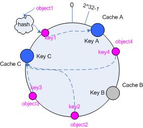
�?/span> 4 Cache B 被移除后�?/span> cache 映射
3.5.2 ��d�� cache
再考虑��d��一台新�?/span> cache D 的情况,假设在这个环�?/span> hash �I�间中, cache D 被映���在对象 object2 �?/span>object3 之间。这时受影响的将仅是那些�?/span> cache D 逆时针遍历直��C��一�?/span> cache �Q?/span> cache B �Q�之间的对象�Q�它们是也本来映���到 cache C 上对象的一部分�Q�,���这些对象重新映���到 cache D 上即可�?/span>
因此�q�里仅需要变动对�?/span> object2 �Q�将光���新映���到 cache D 上;参见�?/span> 5 �?/span>
�?/span> 5 ��d�� cache D 后的映射关系
4 虚拟节点
考量 Hash ���法的另一个指标是�q�����?/span> (Balance) �Q�定义如下:
�q�����?/span>
�q����性是指哈希的�l�果能够���可能分布到所有的�~�冲中去�Q�这样可以��得所有的�~�冲�I�间都得到利用�?/span>
hash ���法�q�不是保证绝对的�q�����Q�如�?/span> cache 较少的话�Q�对象�ƈ不能被均匀的映���到 cache 上,比如在上面的例子中,仅部�|?/span> cache A �?/span> cache C 的情况下�Q�在 4 个对象中�Q?/span> cache A 仅存储了 object1 �Q��?/span> cache C 则存储了 object2 �?/span> object3 �?/span> object4 �Q�分布是很不均衡的�?/span>
��Z��解决�q�种情况�Q?/span> consistent hashing 引入�?#8220;虚拟节点”的概念,它可以如下定义:
“虚拟节点”�Q?/span> virtual node �Q�是实际节点�?/span> hash �I�间的复制品�Q?/span> replica �Q�,一实际个节点对应了若干�?#8220;虚拟节点”�Q�这个对应个��C��成�ؓ“复制个数”�Q?#8220;虚拟节点”�?/span> hash �I�间中以 hash 值排列�?/span>
仍以仅部�|?/span> cache A �?/span> cache C 的情况�ؓ例,在图 4 中我们已�l�看刎ͼ� cache 分布�q�不均匀。现在我们引入虚拟节点,�q�设�|?#8220;复制个数”�?/span> 2 �Q�这���意味着一�׃��存在 4 �?#8220;虚拟节点”�Q?/span> cache A1, cache A2 代表�?/span> cache A �Q?/span> cache C1, cache C2 代表�?/span> cache C �Q�假设一�U�比较理想的情况�Q�参见图 6 �?/span>
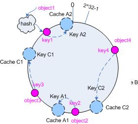
�?/span> 6 引入“虚拟节点”后的映射关系
此时�Q�对象到“虚拟节点”的映���关�p�Mؓ�Q?/span>
objec1->cache A2 �Q?/span> objec2->cache A1 �Q?/span> objec3->cache C1 �Q?/span> objec4->cache C2 �Q?/span>
因此对象 object1 �?/span> object2 都被映射��C�� cache A 上,�?/span> object3 �?/span> object4 映射��C�� cache C 上;�q����性有了很大提高�?/span>
引入“虚拟节点”后,映射关系��׃�� { 对象 -> 节点 } 转换��C�� { 对象 -> 虚拟节点 } 。查询物体所�?/span> cache时的映射关系如图 7 所�C��?/span>
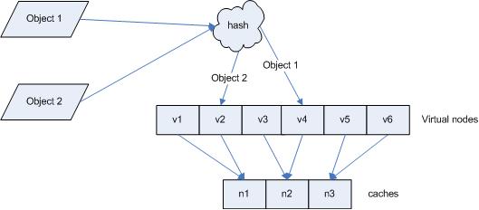
�?/span> 7 查询对象所�?/span> cache
“虚拟节点”�?/span> hash 计算可以采用对应节点�?/span> IP 地址加数字后�~�的方式。例如假�?/span> cache A �?/span> IP 地址�?/span>202.168.14.241 �?/span>
引入“虚拟节点”前,计算 cache A �?/span> hash ��|��
Hash(“202.168.14.241”);
引入“虚拟节点”后,计算“虚拟�?#8221;�?/span> cache A1 �?/span> cache A2 �?/span> hash ��|��
Hash(“202.168.14.241#1”); // cache A1
Hash(“202.168.14.241#2”); // cache A2
5 ���结
Consistent hashing 的基本原理就是这些,具体的分布性等理论分析应该是很复杂的,不过一般也用不到�?/span>
http://weblogs.java.net/blog/2007/11/27/consistent-hashing 上面有一�?/span> java 版本的例子,可以参考�?/span>
http://blog.csdn.net/mayongzhan/archive/2009/06/25/4298834.aspx 转蝲了一�?/span> PHP 版的实现代码�?/span>
http://www.codeproject.com/KB/recipes/lib-conhash.aspx C语言版本
一些参考资料地址�Q?/span>
http://portal.acm.org/citation.cfm?id=258660
http://en.wikipedia.org/wiki/Consistent_hashing
http://www.spiteful.com/2008/03/17/programmers-toolbox-part-3-consistent-hashing/
http://weblogs.java.net/blog/2007/11/27/consistent-hashing
http://tech.idv2.com/2008/07/24/memcached-004/
http://blog.csdn.net/mayongzhan/archive/2009/06/25/4298834.aspx
]]>

每个帖子前面有一个向上的三角形,如果你觉得这个内容很好,���q����M��下,投上一���。根据得���数�Q�系�l�自动统计出热门文章排行榜。但是,�q����得票最多的文章排在�W�一位,�q�要考虑旉���因素�Q�新文章应该比旧文章更容易得到好的排名�?/p>
Hacker News使用Paul Graham开发的Arc语言�~�写�Q�源码可以从arclanguage.org下蝲。它的排名算法是�q�样实现的:

���上面的代码�q�原为数学公式:
其中�Q?/p>
P表示帖子的得���数�Q�减�?是�ؓ了忽略发帖�h的投����?/p>
T表示距离发帖的时��_��单位为小�Ӟ���Q�加�?是�ؓ了防止最新的帖子��D��分母�q�小�Q�之所以选择2�Q�可能是因�ؓ从原始文章出现在其他�|�站�Q�到转脓至Hacker News�Q���^均需要两个小�Ӟ���?/p>
G表示"重力因子"�Q�gravityth power�Q�,卛_��帖子排名往下拉的力量,默认��gؓ1.8�Q�后文会详细讨论�q�个倹{�?/p>
从这个公式来看,军_��帖子排名有三个因素:
�W�一个因素是得票数P�?/strong>
在其他条件不变的情况下,得票���多�Q�排名越高�?/p>

�?a target="_blank" style="margin: 0px; padding: 0px; list-style-type: none; border: none; color: #112233;">上图可以看到�Q�有三个同时发表的帖子,得票分别�?00����?0���和30���(�?后�ؓ199�?9�?9�Q�,分别以黄艌Ӏ���色和蓝色表示。在��M��个时间点上,都是黄色曲线在最上方�Q�蓝色曲�U�在最下方�?/p>
如果你不惌���"高票帖子"�?低票帖子"的差距过大,可以在得���数上加一个小�?的指敎ͼ�比如(P-1)^0.8�?/p>
�W�二个因素是距离发帖的时间T�?/strong>
在其他条件不变的情况下,���是新发表的帖子�Q�排名越高。或者说�Q�一个帖子的排名�Q�会随着旉���不断下降�?/p>
从前一张图可以看到�Q�经�q?4���时之后�Q�所有帖子的得分基本上都���于1�Q�这意味着它们都将跌到排行榜的末尾�Q�保证了排名前列的都���是较新的内宏V�?/p>
�W�三个因素是重力因子G�?/strong>
它的数值大���决定了排名随时间下降的速度�?/p>

�?a target="_blank" style="margin: 0px; padding: 0px; list-style-type: none; border: none; color: #112233;">上图可以看到�Q�三�Ҏ���U�的其他参数都一��P��G的值分别�ؓ1.5�?.8�?.0。G��D��大,曲线���陡峭,排名下降得越快,意味着排行榜的更新速度���快�?/p>
知道了算法的构成�Q�就可以调整参数的��|��以适用你自��q��应用�E�序�?/p>
]]>
惛_��来看�q�篇博文的同学对汉诺塔应该不会陌生了吧,
写这���博�q�是有初��L���Q?/p>
之前学数据结构的时候自��q��书、也上网上查了很多资料,资料都比较散、而且描述的不是很清楚�Q�对于当时刚�?/p>
接触���法的我�Q�要完全理解�q�是有一定难度。今天刚好有旉������整理了下思�\、重写分析了一下之前的疑惑的地斏V�?/p>
没有透彻的地方便都豁然开朗了。所以迫不及待把我的��x��记录下来�Q�和大家分��n�?/p>
如果你也是和之前的我一样对hanoi tower没能完全消化�Q�或者刚刚接触汉诺塔�Q�那希望我的�q�种理解方式能给你些
许帮助,如果你觉得已�l�完全掌握的比较牢靠了,那也可以看看�Q�有好的idea可以一起分享;毕竟交流讨论也是一�U�很好的
学习方式�?/p>
好了�Q�废话不多说�Q�切入正题�?/p>
关于汉诺塔�v源啊、传说啊���马的就不啰嗦了�Q�我们直接切入正题:
问题描述�Q?/p>
有一个梵塔,塔内有三个��A、B、C�Q�A座上有诺�q�个盘子�Q�盘子大���不�{�,大的在下�Q�小的在上(如图�Q��?/p>
把这些个盘子从A座移到C座,中间可以借用B座但每次只能允许�U�d��一个盘子,�q�且在移动过�E�中�Q?个��上的�?/p>
子始�l�保持大盘在下,���盘在上�?/p>
描述���化:把A�׃��的n个盘子移动到C柱,其中可以借用B柱�?/p>

我们直接假设有n个盘子:
先把盘子从小到大标记�?�?�?......n
先看原问题三个柱子的状态:
状�? A�Q�按��序堆放的n个盘子。B:�I�的。C�Q�空的�?/span>
目标是要把A上的n个盘子移动到C。因为必���d��的在下小的在上,所以最�l�结果C盘上最下面的应该是标号为n的盘子,试想�Q?/p>
要取得A上的�W�n个盘子,���p��把它上面的n-1个盘子拿开吧?拿开攑֜�哪里呢?共有三个柱子�Q�A昄���不是、如果放在C�?/p>
了,那么最大的盘子���没地方放,问题�q�是没得到解冟뀂所以选择B柱。当�Ӟ��B上面也是按照大在下小在上的原则堆攄���
�Q�记住:先不要管具体如何�U�d���Q�可以看成用一个函数完成移动,现在不用去考虑函数如何实现。这点很重要�Q��?/strong>
很明显:上一步完成后三个塔的状态:
状�?�Q?nbsp; A�Q�只有最大的一个盘子。B�Q�有按规则堆攄���n-1个盘子。C�I�的�?/span>
上面的很好理解吧�Q�好�Q�其实到�q�里���已�l�完成一半了。(如果前面的没懂,请重看一遍。point�Q�不要管如何�U�d���Q�)
我们�l�箋�Q?/p>
�q�时候,可以直接把A上的最大盘�U�d��到C盘,�U�d��后的状态:
中间状态: A�Q�空的。B�Q�n-1个盘子。C�Q�有一个最大盘�Q�第n个盘子)
要注意的一�Ҏ���Q�这时候的C柱其实可以看做是�I�的。因为剩下的所有盘子都比它���,它们中的��M��一个都可以攑֜�上面�Q�也���是 C�׃���?/p>
所以现在三个柱子的状态:
中间状态: A�Q�空的。B�Q�n-1个盘子。C�Q�空�?/span>
想一惻I��现在的问题和原问题有些相��g��处了吧?。。如何更�怼�呢?。显�Ӟ��只要吧B上的n-1个盘子移动到A�Q�待解决的问题和原问题就相比���只是规模变���了
现在考虑如何把B上的n-1个盘子移动到A上,其实�U�d���Ҏ��和上文中的把n-1个盘从A�U�d��到B是一��L���Q�只是柱子的名称换了下而已。。(如果写成函数�Q�只是参数调用顺序改变而已�Q�。
假设你已�l�完成上一步了�Q�同��L���Q�不要考虑如何�ȝ��动,只要想着用一个函数实现就好)�Q�请看现在的状态:
状�?�Q� A�Q�有按顺序堆攄���n-1个盘子。B�Q�空的。C�Q�按��序堆放的第n盘子(可看为空�?
���在刚才�Q�我们完���的完成了一�ơ递归。如果没看懂请从新看一遍,可以用笔��d��三个状态、静下心来慢慢推理�?/p>
我一再强调的�Q�当要把最大盘子上面的所有盘子移动到另一个空�׃���Ӟ��不要兛_��具体如何�U�d���Q�只用把它看做一个函数可以完成即可,不用兛_��函数的具体实现。如果你的思�\�U�结在这里,���很隄����l�深入了�?/em>
到这里,其实 基本思�\已经理清了。状�?和状�?�Q�除了规模变��?�Q�其它方面没有�Q何区别了。然后只要用相同的思维方式�Q�就能往下深入。。�?/p>
好了�Q�看看如何用���法实现吧:
定义函数Hanoi�Q�a,b,c,n�Q�表�C�把a上的n个盘子移动到c上,其中可以用到b�?/p>
定义函数move(m,n)表示把m上的盘子�U�d��到n�?/p>
我们需要解决的问题正是 Hanoi (a,b,c,n) //上文中的状�?
1、把A上的n-1个移动到B�Q?nbsp; Hanoi (a,c,b,n-1); // 操作�l�束为状�?
2、把A上的大盘子移动到C move(a,c)
3、把B上的n-1�U�d��到A Hanoi (b,c,a,n-1); //操作�l�束位状�?(和状�?相比只是规模变小)
如果现在�q�不能理解、请回过头再看一遍、毕竟如果是初学者不是很�Ҏ�����p��理解的。可以用�W�记下几个关键的状态,�q�且看看你有没有真正的投入去看,独立��L��考了�?/span>
import java.io.IOException;
import java.io.InputStreamReader;
public class Hanoi {
public static void main(String[] args) throws IOException{
int n;
BufferedReader buf;
buf = new BufferedReader(new InputStreamReader(System.in));
System.out.println("Please input the number of disk ");
n = Integer.parseInt(buf.readLine());
Hanoi hanoi = new Hanoi();
hanoi.move(n,'A','B','C');
}
public void move(int n, char a, char b, char c){
if(n == 1){
System.out.println("Disk " + n + " From " + a + " To " + c);
}
else{
move(n-1,a,c,b);
System.out.println("Disk " + n + " From " + a + " To " + c);
move(n-1,b,a,c);
}
}
}
以上、如果有不对的地斏V��还希望您能指出�?/p>
我对递归的一点理解:
解决实际问题时、不能太��d��心实现的�l�节�Q�因为递归的过�E�恰恰是我们实现的方法)���像�q�个问题�Q�如在第一步就�q�多的纠�l�于如何把n-1个盘子移动到B上、那么你的思�\���很隄����l�深入。只要看做是用函数实现就好,如果你能看出不管怎么�U�d���Q�其实本质都一��L��时候,那么���p��较快的得到结果了。就像这个案例,要注意到我们做的关键几步都只是移动的��序有改变,其中的规则没有改变,�?/p>
如果用函数表�C�的话,���只是参数调用的��序有所不同了。在递归的运用中、不用关心每一步的具体实现 �Q�只要看做用一个函数表�C�就好。分析问题的时候,最好画�������q��推理�q�程�Q�得到有效的状态图�?/p>
思考问题讲求思�\的连贯性、力求尽快进入状态,享受完全投入��C��件事中的���妙感觉
]]>
http://renaud.waldura.com/doc/java/dijkstra/
Dijkstra's algorithm is probably the best-known and thus most implemented shortest path algorithm. It is simple, easy to understand and implement, yet impressively efficient. By getting familiar with such a sharp tool, a developer can solve efficiently and elegantly problems that would be considered impossibly hard otherwise. Be my guest as I explore a possible implementation of Dijkstra's shortest path algorithm in Java.
What It Does
Dijkstra's algorithm, when applied to a graph, quickly finds the shortest path from a chosen source to a given destination. (The question "how quickly" is answered later in this article.) In fact, the algorithm is so powerful that it finds all shortest paths from the source to all destinations! This is known as the single-source shortest paths problem. In the process of finding all shortest paths to all destinations, Dijkstra's algorithm will also compute, as a side-effect if you will, a spanning tree for the graph. While an interesting result in itself, the spanning tree for a graph can be found using lighter (more efficient) methods than Dijkstra's.
How It Works
First let's start by defining the entities we use. The graph is made of vertices (or nodes, I'll use both words interchangeably), and edges which link vertices together. Edges are directed and have an associated distance, sometimes called the weight or the cost. The distance between the vertex u and the vertex v is noted [u, v] and is always positive.

Dijkstra's algorithm partitions vertices in two distinct sets, the set of unsettled vertices and the set of settled vertices. Initially all vertices are unsettled, and the algorithm ends once all vertices are in the settled set. A vertex is considered settled, and moved from the unsettled set to the settled set, once its shortest distance from the source has been found.
We all know that algorithm + data structures = programs, in the famous words of Niklaus Wirth. The following data structures are used for this algorithm:
| d | stores the best estimate of the shortest distance from the source to each vertex |
|---|---|
| π | stores the predecessor of each vertex on the shortest path from the source |
| S | the set of settled vertices, the vertices whose shortest distances from the source have been found |
| Q | the set of unsettled vertices |
With those definitions in place, a high-level description of the algorithm is deceptively simple. With s as the source vertex:
while Q is not empty {
u = extract-minimum(Q)
add u to S
relax-neighbors(u)
}
Dead simple isn't it? The two procedures called from the main loop are defined below:
for each vertex v adjacent to u, v not in S
{
if d(v) > d(u) + [u,v]
// a shorter distance exists
{
d(v) = d(u) + [u,v]
π(v) = u
add v to Q
}
}
}
extract-minimum(Q) {
find the smallest (as defined by d) vertex in Q
remove it from Q and return it
}
An Example
So far I've listed the instructions that make up the algorithm. But to really understand it, let's follow the algorithm on an example. We shall run Dikjstra's shortest path algorithm on the following graph, starting at the source vertex a.

We start off by adding our source vertex a to the set Q. Q isn't empty, we extract its minimum, a again. We add a to S, then relax its neighbors. (I recommend you follow the algorithm in parallel with this explanation.)

Those neighbors, vertices adjacent to a, are b and c (in green above). We first compute the best distance estimate from a to b. d(b) was initialized to infinity, therefore we do:
d(b) = d(a) + [a,b] = 0 + 4 = 4π(b) is set to a, and we add b to Q. Similarily for c, we assign d(c) to 2, and π(c) to a. Nothing tremendously exciting so far.
The second time around, Q contains b and c. As seen above, c is the vertex with the current shortest distance of 2. It is extracted from the queue and added to S, the set of settled nodes. We then relax the neighbors of c, which are b, d and a.

a is ignored because it is found in the settled set. But it gets interesting: the first pass of the algorithm had concluded that the shortest path from a to b was direct. Looking at c's neighbor b, we realize that:
d(b) = 4 > d(c) + [c,b] = 2 + 1 = 3Ah-ah! We have found that a shorter path going through c exists between a and b. d(b) is updated to 3, and π(b) updated to c. b is added again to Q. The next adjacent vertex is d, which we haven't seen yet. d(d) is set to 7 and π(d) to c.
The unsettled vertex with the shortest distance is extracted from the queue, it is now b. We add it to the settled set and relax its neighbors c and d.

We skip c, it has already been settled. But a shorter path is found for d:
d(d) = 7 > d(b) + [b,d] = 3 + 1 = 4Therefore we update d(d) to 4 and π(d) to b. We add d to the Q set.
At this point the only vertex left in the unsettled set is d, and all its neighbors are settled. The algorithm ends. The final results are displayed in red below:
- π - the shortest path, in predecessor fashion
- d - the shortest distance from the source for each vertex

This completes our description of Dijkstra's shortest path algorithm. Other shortest path algorithms exist (see the References section at the end of this article), but Dijkstra's is one of the simplest, while still offering good performance in most cases.
Implementing It in Java
The Java implementation is quite close to the high-level description we just walked through. For the purpose of this article, my Java implementation of Dijkstra's shortest path finds shortest routes between cities on a map. The RoutesMap object defines a weighted, oriented graph as defined in the introduction section of this article.
int getDistance(City start, City end);
List<City> getDestinations(City city);
}
Data Structures
We've listed above the data structures used by the algorithm, let's now decide how we are going to implement them in Java.
S, the settled nodes set
This one is quite straightforward. The Java Collections feature the Set interface, and more precisely, the HashSet implementation which offers constant-time performance on the contains operation, the only one we need. This defines our first data structure.
private boolean isSettled(City v) {
return settledNodes.contains(v);
}
Notice how my data structure is declared as an abstract type (Set) instead of a concrete type (HashSet). Doing so is a good software engineering practice, as it allows to change the actual type of the collection without any modification to the code that uses it.
d, the shortest distances list
As we've seen, one output of Dijkstra's algorithm is a list of shortest distances from the source node to all the other nodes in the graph. A straightforward way to implement this in Java is with a Map, used to keep the shortest distance value for every node. We also define two accessors for readability, and to encapsulate the default infinite distance.
private void setShortestDistance(City city, int distance) {
shortestDistances.put(city, distance);
}
public int getShortestDistance(City city) {
Integer d = shortestDistances.get(city);
return (d == null) ? INFINITE_DISTANCE : d;
}
You may notice I declare this field final. This is a Java idiom used to flag aggregation relationships between objects. By marking a field final, I am able to convey that it is part of a aggregation relationship, enforced by the properties of final—the encapsulating class cannot exist without this field.
π, the predecessors tree
Another output of the algorithm is the predecessors tree, a tree spanning the graph which yields the actual shortest paths. Because this is the predecessors tree, the shortest paths are actually stored in reverse order, from destination to source. Reversing a given path is easy with Collections.reverse().
The predecessors tree stores a relationship between two nodes, namely a given node's predecessor in the spanning tree. Since this relationship is one-to-one, it is akin to amapping between nodes. Therefore it can be implemented with, again, a Map. We also define a pair of accessors for readability.
private void setPredecessor(City a, City b) {
predecessors.put(a, b);
}
public City getPredecessor(City city) {
return predecessors.get(city);
}
Again I declare my data structure to be of the abstract type Map, instead of the concrete type HashMap. And tag it final as well.
Q, the unsettled nodes set
As seen in the previous section, a data structure central to Dijkstra's algorithm is the set of unsettled vertices Q. In Java programming terms, we need a structure able to store the nodes of our example graph, i.e. City objects. That structure is then looked up for the city with the current shortest distance given by d().
We could do this by using another Set of cities, and sort it according to d() to find the city with shortest distance every time we perform this operation. This isn't complicated, and we could leverage Collections.min() using a custom Comparator to compare the elements according to d().
But because we do this at every iteration, a smarter way would be to keep the set ordered at all times. That way all we need to do to get the city with the lowest distance is to get the first element in the set. New elements would need to be inserted in the right place, so that the set is always kept ordered.
A quick search through the Java collections API yields the PriorityQueue: it can sort elements according to a custom comparator, and provides constant-time access to the smallest element. This is precisely what we need, and we'll write a comparator to order cities (the set elements) according to the current shortest distance. Such a comparator is included below, along with the PriorityQueue definition. Also listed is the small method that extracts the node with the shortest distance.
{
public int compare(City left, City right)
{
int shortestDistanceLeft = getShortestDistance(left);
int shortestDistanceRight = getShortestDistance(right);
if (shortestDistanceLeft > shortestDistanceRight)
{
return +1;
}
else if (shortestDistanceLeft < shortestDistanceRight)
{
return -1;
}
else // equal
{
return left.compareTo(right);
}
}
};
private final PriorityQueue<City> unsettledNodes = new PriorityQueue<City>(INITIAL_CAPACITY, shortestDistanceComparator);
private City extractMin()
{
return unsettledNodes.poll();
}
One important note about the comparator: it is used by the PriorityQueue to determine both object ordering and identity. If the comparator returns that two elements are equal, the queue infers they are the same, and it stores only one instance of the element. To prevent losing nodes with equal shortest distances, we must compare the elements themselves (third block in the if statement above).
Having powerful, flexible data structures at our disposal is what makes Java such an enjoyable language (that, and garbage collection of course).
Putting It All Together
We have defined our data structures, we understand the algorithm, all that remains to do is implement it. As I mentioned earlier, my implementation is close to the high-level description given above. Note that when the only shortest path between two specific nodes is asked, the algorithm can be interrupted as soon as the destination node is reached.
initDijkstra(start);
while (!unsettledNodes.isEmpty()) {
// get the node with the shortest distance
City u = extractMin();
// destination reached, stop
if (u == destination) break;
settledNodes.add(u);
relaxNeighbors(u);
}
}
The DijkstraEngine class implements this algorithm and brings it all together. See "Implementation Notes" below to download the source code.
A Word About Performance
The complexity of Dijkstra's algorithm depends heavily on the complexity of the priority queue Q. If this queue is implemented naively as I first introduced it (i.e. it is re-ordered at every iteration to find the mininum node), the algorithm performs in O(n2), where n is the number of nodes in the graph.
With a real priority queue kept ordered at all times, as we implemented it, the complexity averages O(n log m). The logarithm function stems from the collectionsPriorityQueue class, a heap implementation which performs in log(m).
Implementation Notes
The Java source code discussed in this article is available for download as a ZIP file. Extensive unit tests are provided and validate the correctness of the implementation. Some minimal Javadoc is also provided. As the code makes use of the assert facility and generics, it must be compiled with "javac -source 1.5"; the tests require junit.jar.I warmly recommend Eclipse for all Java development.
I've received a fair amount of e-mail about this article, which has become quite popular. I'm unfortunately unable to answer all your questions, and for this I apologize. Keep in mind this article (and the code) is meant as a starting point: the implementation discussed here is hopefully simple, correct, and relatively easy to understand, but is probably not suited to your specific problem. You must tailor it to your own domain.
My goal in writing this article was to share and teach a useful tool, striving for 1- simplicity and 2- correctness. I purposefully shied away from turning this exercise into a full-blown generic Java implementation. Readers after full-featured, industrial-strength Java implementations of Dijkstra's shortest path algorithm should look at the "Resources" section below.
]]>
APIs.
We define the APIs for bags, queues, and stacks. Beyond the basics, these APIs reflect two Java features: generics and iterable collections.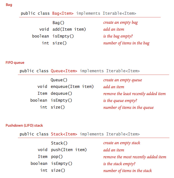
- Generics. An essential characteristic of collection ADTs is that we should be able to use them for any type of data. A specific Java mechanism known as generics enables this capability. The notation <Item> after the class name in each of our APIs defines the name Item as a type parameter, a symbolic placeholder for some concrete type to be used by the client. You can read Stack<Item> as "stack of items." For example, you can write code such as
to use a stack for String objects.Stack<String> stack = new Stack<String>();
stack.push("Test");
...
String next = stack.pop(); - Autoboxing. Type parameters have to be instantiated as reference types, so Java automatically converts between a primitive type and its corresponding wrapper type in assignments, method arguments, and arithmetic/logic expressions. This conversion enables us to use generics with primitive types, as in the following code:
Automatically casting a primitive type to a wrapper type is known as autoboxing, and automatically casting a wrapper type to a primitive type is known as auto-unboxing.Stack<Integer> stack = new Stack<Integer>(); stack.push(17);
// auto-boxing (int -> Integer) int i = stack.pop();
// auto-unboxing (Integer -> int) - Iterable collections. For many applications, the client's requirement is just to process each of the items in some way, or to iterate through the items in the collection. Java's foreach statement supports this paradigm. For example, suppose that collection is a Queue<Transaction>. Then, if the collection is iterable, the client can print a transaction list with a single statement:
for (Transaction t : collection)
StdOut.println(t); - Bags. A bag is a collection where removing items is not supported—its purpose is to provide clients with the ability to collect items and then to iterate through the collected items. Stats.java is a bag client that reads a sequence of real numbers from standard input and prints out their mean and standard deviation.
- FIFO queues. A FIFO queue is a collection that is based on the first-in-first-out (FIFO) policy. The policy of doing tasks in the same order that they arrive server is one that we encounter frequently in everyday life: from people waiting in line at a theater, to cars waiting in line at a toll booth, to tasks waiting to be serviced by an application on your computer.
- Pushdown stack. A pushdown stack is a collection that is based on the last-in-first-out (LIFO) policy. When you click a hyperlink, your browser displays the new page (and pushes onto a stack). You can keep clicking on hyperlinks to visit new pages, but you can always revisit the previous page by clicking the back button (popping it from the stack). Reverse.java is a stack client that reads a sequence of integers from standard input and prints them in reverse order.
- Arithmetic expression evaluation. Evaluate.java is a stack client that evaluates fully parenthesized arithmetic expressions. It uses Dijkstra's 2-stack algorithm:
- Push operands onto the operand stack.
- Push operators onto the operator stack.
- Ignore left parentheses.
- On encountering a right parenthesis, pop an operator, pop the requisite number of operands, and push onto the operand stack the result of applying that operator to those operands.
This code is a simple example of an interpreter.
Array and resizing array implementations of collections.
- Fixed-capacity stack of strings. FixedCapacityStackOfString.java implements a fixed-capacity stack of strings using an array.
- Fixed-capacity generic stack. FixedCapacityStack.java implements a generic fixed-capacity stack.
- Array resizing stack. ResizingArrayStack.java implements a generic stack using a resizing array. With a resizing array, we dynamically adjust the size of the array so that it is both sufficiently large to hold all of the items and not so large as to waste an excessive amount of space. Wedouble the size of the array in push() if it is full; we halve the size of the array in pop() if it is less than one-quarter full.
- Array resizing queue. ResizingArrayQueue.java implements the queue API with a resizing array.
Linked lists.
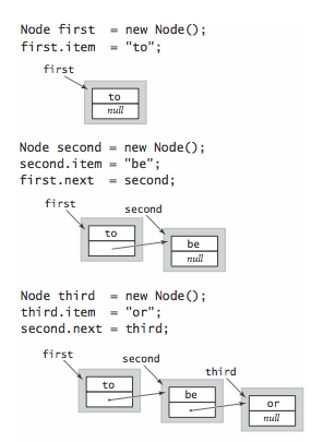
A linked list is a recursive data structure that is either empty (null) or a reference to a node having a generic item and a reference to a linked list. To implement a linked list, we start with a nested class that defines the node abstraction
private class Node {
    Item item;
    Node next;
 }
- Building a linked list. To build a linked list that contains the items to, be, and or, we create a Node for each item, set the item field in each of th
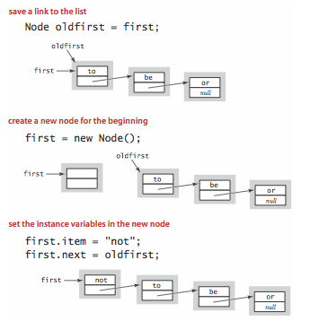
- Insert at the beginning. The easiest place to insert a new node in a linked list is at the beginning.
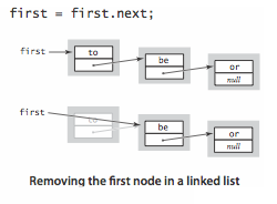
- Remove from the beginning. Removing the first node in a linked list is also easy.
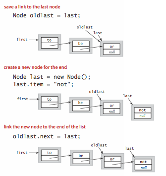
- Insert at the end. To insert a node at the end of a linked list, we maintain a link to the last node in the list.
- Traversal. The following is the idiom for traversing the nodes in a linked list.
for (Node x = first; x != null; x = x.next) {
    // process x.item
 }
Linked-list implementations of collections.
- Linked list implementation of a stack. Stack.java implements a generic stack using a linked list. It maintains the stack as a linked list, with the top of the stack at the beginning, referenced by an instance variable first. To push() an item, we add it to the beginning of the list; to pop()an item, we remove it from the beginning of the list.
- Linked list implementation of a queue. Program Queue.java implements a generic FIFO queue using a linked list. It maintains the queue as a linked list in order from least recently to most recently added items, with the beginning of the queue referenced by an instance variable firstand the end of the queue referenced by an instance variable last. To enqueue() an item, we add it to the end of the list; to dequeue() an item, we remove it from the beginning of the list.
- Linked list implementation of a bag. Program Bag.java implements a generic bag using a linked list. The implementation is the same as Stack.javaexcept for changing the name of push() to add() and removing pop().
Iteration.
To consider the task of implementing iteration, we start with a snippet of client code that prints all of the items in a collection of strings, one per line:This foreach statement is shorthand for the following while statement:
...
for (String s : collection)
StdOut.println(s);
...
To implement iteration in a collection:
while (i.hasNext()) {
String s = i.next();
StdOut.println(s);
}
- Include the following import statement so that our code can refer to Java's java.util.Iterator interface:
import java.util.Iterator;
- Add the following to the class declaration, a promise to provide an iterator() method, as specified in the java.lang.Iterable interface:
implements Iterable<Item>
- Implement a method iterator() that returns an object from a class that implements the Iterator interface:
public Iterator<Item> iterator() {
     return new ListIterator();
} - Implement a nested class that implements the Iterator interface by including the methods hasNext(), next(), and remove(). We always use an empty method for the optional remove() method because interleaving iteration with operations that modify the data structure is best avoided.
- The nested class ListIterator in Bag.java illustrates how to implement a class that implements the Iterator interface when the underlying data structure is a linked list.
- The nested class ArrayIterator in ArrayResizingBag.java does the same when the underlying data structure is an array.
Autoboxing Q + A
Q. How does auto-boxing handle the following code fragment?
A. It results in a run-time error. Primitive type can store every value of their corresponding wrapper type except null.
Q. Why does the first group of statements print true, but the second false?
Integer a2 = 100;
System.out.println(a1 == a2);
// true Integer b1 = new Integer(100);
Integer b2 = new Integer(100);
System.out.println(b1 == b2);
// false Integer c1 = 150;
Integer c2 = 150;
System.out.println(c1 == c2);
// false
A. The second prints false because b1 and b2 are references to different Integer objects. The first and third code fragments rely on autoboxing. Surprisingly the first prints true because values between -128 and 127 appear to refer to the same immutable Integer objects (Java's implementation of valueOf() retrieves a cached values if the integer is between -128 and 127), while Java constructs new objects for each integer outside this range.
Here is another Autoboxing.java anomaly.
Generics Q + A
Q. Are generics solely for auto-casting?
A. No, but we will use them only for "concrete parameterized types", where each data type is parameterized by a single type. The primary benefit is to discover type mismatch errors at compile-time instead of run-time. There are other more general (and more complicated) uses of generics, including wildcards. This generality is useful for handling subtypes and inheritance. For more information, see this Generics FAQ and this generics tutorial.
Q. Can concrete parameterized types be used in the same way as normal types?
A. Yes, with a few exceptions (array creation, exception handling, with instanceof, and in a class literal).
Q. Why do I get a "can't create an array of generics" error when I try to create an array of generics?
public class ResizingArrayStack<Item> {
    Item[] a = new Item[1];
}
A. Unfortunately, creating arrays of generics is not possible in Java 1.5. The underlying cause is that arrays in Java are covariant, but generics are not. In other words, String[] is a subtype of Object[], but Stack<String> is not a subtype of Stack<Object>. To get around this defect, you need to perform an unchecked cast as in ResizingArrayStack.java.
Q. So, why are arrays covariant?
A. Many programmers (and programming language theorists) consider covariant arrays to be a serious defect in Java's type system: they incur unnecessary run-time performance overhead (for example, see ArrayStoreException) and can lead to subtle bugs. Covariant arrays were introduced in Java to circumvent the problem that Java didn't originally include generics in its design, e.g., to implement Arrays.sort(Comparable[]) and have it be callable with an input array of type String[].
Q. Can I create and return a new array of a parameterized type, e.g., to implement a toArray() method for a generic queue?
A. Not easily. You can do it using reflection provided that the client passes an object of the desired concrete type to toArray() This is the (awkward) approach taken by Java's Collection Framework.
]]>
public static int BUFFERSIZE = 2048;
public BufferedReader fbr;
public File originalfile;
private String cache;
private boolean empty;
public BinaryFileBuffer(File f, Charset cs) throws IOException {
originalfile = f;
fbr = new BufferedReader(new InputStreamReader(new FileInputStream(f), cs), BUFFERSIZE);
reload();
}
public boolean empty() {
return empty;
}
private void reload() throws IOException {
try {
if ((this.cache = fbr.readLine()) == null) {
empty = true;
cache = null;
} else {
empty = false;
}
} catch (EOFException oef) {
empty = true;
cache = null;
}
}
public void close() throws IOException {
fbr.close();
}
public String peek() {
if (empty())
return null;
return cache.toString();
}
public String pop() throws IOException {
String answer = peek();
reload();
return answer;
}
}
]]>
]]>