|
|
2011年3月15日
不同的平臺,內(nèi)存模型是不一樣的,但是jvm的內(nèi)存模型規(guī)范是統(tǒng)一的。其實(shí)java的多線程并發(fā)問題最終都會反映在java的內(nèi)存模型上,所謂線程安全無 非是要控制多個線程對某個資源的有序訪問或修改。總結(jié)java的內(nèi)存模型,要解決兩個主要的問題:可見性和有序性。我們都知道計(jì)算機(jī)有高速緩存的存在,處 理器并不是每次處理數(shù)據(jù)都是取內(nèi)存的。JVM定義了自己的內(nèi)存模型,屏蔽了底層平臺內(nèi)存管理細(xì)節(jié),對于java開發(fā)人員,要清楚在jvm內(nèi)存模型的基礎(chǔ) 上,如果解決多線程的可見性和有序性。
那么,何謂可見性? 多個線程之間是不能互相傳遞數(shù)據(jù)通信的,它們之間的溝通只能通過共享變量來進(jìn)行。Java內(nèi)存模型(JMM)規(guī)定了jvm有主內(nèi)存,主內(nèi)存是多個線程共享 的。當(dāng)new一個對象的時候,也是被分配在主內(nèi)存中,每個線程都有自己的工作內(nèi)存,工作內(nèi)存存儲了主存的某些對象的副本,當(dāng)然線程的工作內(nèi)存大小是有限制 的。當(dāng)線程操作某個對象時,執(zhí)行順序如下:
(1) 從主存復(fù)制變量到當(dāng)前工作內(nèi)存 (read and load)
(2) 執(zhí)行代碼,改變共享變量值 (use and assign)
(3) 用工作內(nèi)存數(shù)據(jù)刷新主存相關(guān)內(nèi)容 (store and write) JVM規(guī)范定義了線程對主存的操作指 令:read,load,use,assign,store,write。當(dāng)一個共享變量在多個線程的工作內(nèi)存中都有副本時,如果一個線程修改了這個共享 變量,那么其他線程應(yīng)該能夠看到這個被修改后的值,這就是多線程的可見性問題。
那么,什么是有序性呢 ?線程在引用變量時不能直接從主內(nèi)存中引用,如果線程工作內(nèi)存中沒有該變量,則會從主內(nèi)存中拷貝一個副本到工作內(nèi)存中,這個過程為read-load,完 成后線程會引用該副本。當(dāng)同一線程再度引用該字段時,有可能重新從主存中獲取變量副本(read-load-use),也有可能直接引用原來的副本 (use),也就是說 read,load,use順序可以由JVM實(shí)現(xiàn)系統(tǒng)決定。
線程不能直接為主存中中字段賦值,它會將值指定給工作內(nèi)存中的變量副本(assign),完成后這個變量副本會同步到主存儲區(qū)(store- write),至于何時同步過去,根據(jù)JVM實(shí)現(xiàn)系統(tǒng)決定.有該字段,則會從主內(nèi)存中將該字段賦值到工作內(nèi)存中,這個過程為read-load,完成后線 程會引用該變量副本,當(dāng)同一線程多次重復(fù)對字段賦值時,比如:
Java代碼
for(int i=0;i<10;i++)
a++;
線程有可能只對工作內(nèi)存中的副本進(jìn)行賦值,只到最后一次賦值后才同步到主存儲區(qū),所以assign,store,weite順序可以由JVM實(shí)現(xiàn)系統(tǒng)決 定。假設(shè)有一個共享變量x,線程a執(zhí)行x=x+1。從上面的描述中可以知道x=x+1并不是一個原子操作,它的執(zhí)行過程如下:
1 從主存中讀取變量x副本到工作內(nèi)存
2 給x加1
3 將x加1后的值寫回主 存
如果另外一個線程b執(zhí)行x=x-1,執(zhí)行過程如下:
1 從主存中讀取變量x副本到工作內(nèi)存
2 給x減1
3 將x減1后的值寫回主存
那么顯然,最終的x的值是不可靠的。假設(shè)x現(xiàn)在為10,線程a加1,線程b減1,從表面上看,似乎最終x還是為10,但是多線程情況下會有這種情況發(fā)生:
1:線程a從主存讀取x副本到工作內(nèi)存,工作內(nèi)存中x值為10
2:線程b從主存讀取x副本到工作內(nèi)存,工作內(nèi)存中x值為10
3:線程a將工作內(nèi)存中x加1,工作內(nèi)存中x值為11
4:線程a將x提交主存中,主存中x為11
5:線程b將工作內(nèi)存中x值減1,工作內(nèi)存中x值為9
6:線程b將x提交到中主存中,主存中x為 jvm的內(nèi)存模型之eden區(qū)所謂線程的“工作內(nèi)存”到底是個什么東西?有的人認(rèn)為是線程的棧,其實(shí)這種理解是不正確的。看看JLS(java語言規(guī)范)對線程工作 內(nèi)存的描述,線程的working memory只是cpu的寄存器和高速緩存的抽象描述。 可能 很多人都覺得莫名其妙,說JVM的內(nèi)存模型,怎么會扯到cpu上去呢?在此,我認(rèn)為很有必要闡述下,免 得很多人看得不明不白的。先拋開java虛擬機(jī)不談,我們都知道,現(xiàn)在的計(jì)算機(jī),cpu在計(jì)算的時候,并不總是從內(nèi)存讀取數(shù)據(jù),它的數(shù)據(jù)讀取順序優(yōu)先級 是:寄存器-高速緩存-內(nèi)存。線程耗費(fèi)的是CPU,線程計(jì)算的時候,原始的數(shù)據(jù)來自內(nèi)存,在計(jì)算過程中,有些數(shù)據(jù)可能被頻繁讀取,這些數(shù)據(jù)被存儲在寄存器 和高速緩存中,當(dāng)線程計(jì)算完后,這些緩存的數(shù)據(jù)在適當(dāng)?shù)臅r候應(yīng)該寫回內(nèi)存。當(dāng)個多個線程同時讀寫某個內(nèi)存數(shù)據(jù)時,就會產(chǎn)生多線程并發(fā)問題,涉及到三個特 性:原子性,有序性,可見性。在《線程安全總結(jié)》這篇文章中,為了理解方便,我把原子性和有序性統(tǒng)一叫做“多線程執(zhí)行有序性”。支持多線程的平臺都會面臨 這種問題,運(yùn)行在多線程平臺上支持多線程的語言應(yīng)該提供解決該問題的方案。 synchronized, volatile,鎖機(jī)制(如同步塊,就緒隊(duì) 列,阻塞隊(duì)列)等等。這些方案只是語法層面的,但我們要從本質(zhì)上去理解它,不能僅僅知道一個 synchronized 可以保證同步就完了。 在這里我說的是jvm的內(nèi)存模型,是動態(tài)的,面向多線程并發(fā)的,沿襲JSL的“working memory”的說法,只是不想牽扯到太多底層細(xì)節(jié),因?yàn)?《線程安全總結(jié)》這篇文章意在說明怎樣從語法層面去理解java的線程同步,知道各個關(guān)鍵字的使用場 景。 說說JVM的eden區(qū)吧。JVM的內(nèi)存,被劃分了很多的區(qū)域: 1.程序計(jì)數(shù)器
每一個Java線程都有一個程序計(jì)數(shù)器來用于保存程序執(zhí)行到當(dāng)前方法的哪一個指令。
2.線程棧
線程的每個方法被執(zhí)行的時候,都會同時創(chuàng)建一個幀(Frame)用于存儲本地變量表、操作棧、動態(tài)鏈接、方法出入口等信息。每一個方法的調(diào)用至完成,就意味著一個幀在VM棧中的入棧至出棧的過程。如果線程請求的棧深度大于虛擬機(jī)所允許的深度,將拋出StackOverflowError異常;如果VM棧可以動態(tài)擴(kuò)展(VM Spec中允許固定長度的VM棧),當(dāng)擴(kuò)展時無法申請到足夠內(nèi)存則拋出OutOfMemoryError異常。
3.本地方法棧
4.堆
每個線程的棧都是該線程私有的,堆則是所有線程共享的。當(dāng)我們new一個對象時,該對象就被分配到了堆中。但是堆,并不是一個簡單的概念,堆區(qū)又劃分了很多區(qū)域,為什么堆劃分成這么多區(qū)域,這是為了JVM的內(nèi)存垃圾收集,似乎越扯越遠(yuǎn)了,扯到垃圾收集了,現(xiàn)在的jvm的gc都是按代收集,堆區(qū)大致被分為三大塊:新生代,舊生代,持久代(虛擬的);新生代又分為eden區(qū),s0區(qū),s1區(qū)。新建一個對象時,基本小的對象,生命周期短的對象都會放在新生代的eden區(qū)中,eden區(qū)滿時,有一個小范圍的gc(minor gc),整個新生代滿時,會有一個大范圍的gc(major gc),將新生代里的部分對象轉(zhuǎn)到舊生代里。
5.方法區(qū)
其實(shí)就是永久代(Permanent Generation),方法區(qū)中存放了每個Class的結(jié)構(gòu)信息,包括常量池、字段描述、方法描述等等。VM Space描述中對這個區(qū)域的限制非常寬松,除了和Java堆一樣不需要連續(xù)的內(nèi)存,也可以選擇固定大小或者可擴(kuò)展外,甚至可以選擇不實(shí)現(xiàn)垃圾收集。相對來說,垃圾收集行為在這個區(qū)域是相對比較少發(fā)生的,但并不是某些描述那樣永久代不會發(fā)生GC(至 少對當(dāng)前主流的商業(yè)JVM實(shí)現(xiàn)來說是如此),這里的GC主要是對常量池的回收和對類的卸載,雖然回收的“成績”一般也比較差強(qiáng)人意,尤其是類卸載,條件相當(dāng)苛刻。
6.常量池
Class文件中除了有類的版本、字段、方法、接口等描述等信息外,還有一項(xiàng)信息是常量表(constant_pool table),用于存放編譯期已可知的常量,這部分內(nèi)容將在類加載后進(jìn)入方法區(qū)(永久代)存放。但是Java語言并不要求常量一定只有編譯期預(yù)置入Class的常量表的內(nèi)容才能進(jìn)入方法區(qū)常量池,運(yùn)行期間也可將新內(nèi)容放入常量池(最典型的String.intern()方法)。
ArrayList 關(guān)于 Java中的transient,volatile和strictfp關(guān)鍵字 http://www.iteye.com/topic/52957 (1), ArrayList底層使用Object數(shù)據(jù)實(shí)現(xiàn), private transient Object[] elementData;且在使用不帶參數(shù)的方式實(shí)例化時,生成數(shù)組默認(rèn)的長度是10。 (2), add方法實(shí)現(xiàn) public boolean add(E e) {
//ensureCapacityInternal判斷添加新元素是否需要重新擴(kuò)大數(shù)組的長度,需要則擴(kuò)否則不 ensureCapacityInternal(size + 1); // 此為JDK7調(diào)用的方法 JDK5里面使用的ensureCapacity方法 elementData[size++] = e; //把對象插入數(shù)組,同時把數(shù)組存儲的數(shù)據(jù)長度size加1 return true; } JDK 7中 ensureCapacityInternal實(shí)現(xiàn) private void ensureCapacityInternal(int minCapacity) { modCount++;修改次數(shù) // overflow-conscious code if (minCapacity - elementData.length > 0) grow(minCapacity);//如果需要擴(kuò)大數(shù)組長度 } /** * The maximum size of array to allocate. --申請新數(shù)組最大長度 * Some VMs reserve some header words in an array. * Attempts to allocate larger arrays may result in * OutOfMemoryError: Requested array size exceeds VM limit --如果申請的數(shù)組占用的內(nèi)心大于JVM的限制拋出異常 */ private static final int MAX_ARRAY_SIZE = Integer.MAX_VALUE - 8;//為什么減去8看注釋第2行 /** * Increases the capacity to ensure that it can hold at least the * number of elements specified by the minimum capacity argument. * * @param minCapacity the desired minimum capacity */ private void grow(int minCapacity) { // overflow-conscious code int oldCapacity = elementData.length; int newCapacity = oldCapacity + (oldCapacity >> 1); //新申請的長度為old的3/2倍同時使用位移運(yùn)算更高效,JDK5中: (oldCapacity *3)/2+1 if (newCapacity - minCapacity < 0) newCapacity = minCapacity; if (newCapacity - MAX_ARRAY_SIZE > 0) //你懂的 newCapacity = hugeCapacity(minCapacity); // minCapacity is usually close to size, so this is a win: elementData = Arrays.copyOf(elementData, newCapacity); } //可以申請的最大長度 private static int hugeCapacity(int minCapacity) { if (minCapacity < 0) // overflow throw new OutOfMemoryError(); return (minCapacity > MAX_ARRAY_SIZE) ? Integer.MAX_VALUE : MAX_ARRAY_SIZE; }
Quicksort
Quicksort is a fast sorting algorithm, which is used not only for educational purposes, but widely applied in practice. On the average, it has O(n log n) complexity, making quicksort suitable for sorting big data volumes. The idea of the algorithm is quite simple and once you realize it, you can write quicksort as fast as bubble sort.
Algorithm
The divide-and-conquer strategy is used in quicksort. Below the recursion step is described:
- Choose a pivot value. We take the value of the middle element as pivot value, but it can be any value, which is in range of sorted values, even if it doesn't present in the array.
- Partition. Rearrange elements in such a way, that all elements which are lesser than the pivot go to the left part of the array and all elements greater than the pivot, go to the right part of the array. Values equal to the pivot can stay in any part of the array. Notice, that array may be divided in non-equal parts.
- Sort both parts. Apply quicksort algorithm recursively to the left and the right parts.
Partition algorithm in detail
There are two indices i and j and at the very beginning of the partition algorithm i points to the first element in the array andj points to the last one. Then algorithm moves i forward, until an element with value greater or equal to the pivot is found. Index j is moved backward, until an element with value lesser or equal to the pivot is found. If i ≤ j then they are swapped and i steps to the next position (i + 1), j steps to the previous one (j - 1). Algorithm stops, when i becomes greater than j.
After partition, all values before i-th element are less or equal than the pivot and all values after j-th element are greater or equal to the pivot.
Example. Sort {1, 12, 5, 26, 7, 14, 3, 7, 2} using quicksort.
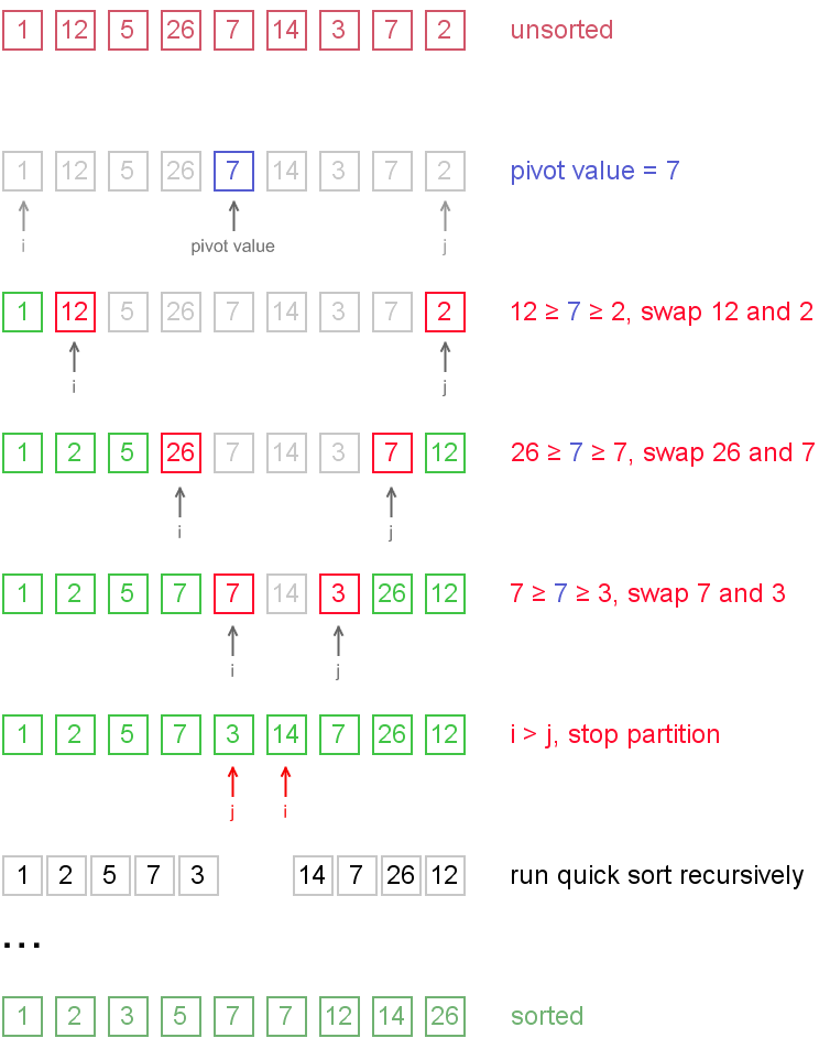
Notice, that we show here only the first recursion step, in order not to make example too long. But, in fact, {1, 2, 5, 7, 3} and {14, 7, 26, 12} are sorted then recursively.
Why does it work?
On the partition step algorithm divides the array into two parts and every element a from the left part is less or equal than every element b from the right part. Also a and b satisfy a ≤ pivot ≤ b inequality. After completion of the recursion calls both of the parts become sorted and, taking into account arguments stated above, the whole array is sorted.
Complexity analysis
On the average quicksort has O(n log n) complexity, but strong proof of this fact is not trivial and not presented here. Still, you can find the proof in [1]. In worst case, quicksort runs O(n2) time, but on the most "practical" data it works just fine and outperforms other O(n log n) sorting algorithms.
Code snippets
Java
int partition(int arr[], int left, int right)
{
int i = left;
int j = right;
int temp;
int pivot = arr[(left+right)>>1];
while(i<=j){
while(arr[i]>=pivot){
i++;
}
while(arr[j]<=pivot){
j--;
}
if(i<=j){
temp = arr[i];
arr[i] = arr[j];
arr[j] = temp;
i++;
j--;
}
}
return i
}
void quickSort(int arr[], int left, int right) {
int index = partition(arr, left, right);
if(left<index-1){
quickSort(arr,left,index-1);
}
if(index<right){
quickSort(arr,index,right);
}
}
python
def quickSort(L,left,right) {
i = left
j = right
if right-left <=1:
return L
pivot = L[(left + right) >>1];
/* partition */
while (i <= j) {
while (L[i] < pivot)
i++;
while (L[j] > pivot)
j--;
if (i <= j) {
L[i],L[j] = L[j],L[i]
i++;
j--;
}
};
/* recursion */
if (left < j)
quickSort(L, left, j);
if (i < right)
quickSort(L, i, right);
}
|
Insertion Sort
Insertion sort belongs to the O(n2) sorting algorithms. Unlike many sorting algorithms with quadratic complexity, it is actually applied in practice for sorting small arrays of data. For instance, it is used to improve quicksort routine. Some sources notice, that people use same algorithm ordering items, for example, hand of cards.
Algorithm
Insertion sort algorithm somewhat resembles selection sort. Array is imaginary divided into two parts - sorted one andunsorted one. At the beginning, sorted part contains first element of the array and unsorted one contains the rest. At every step, algorithm takes first element in the unsorted part and inserts it to the right place of the sorted one. Whenunsorted part becomes empty, algorithm stops. Sketchy, insertion sort algorithm step looks like this:
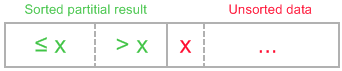
becomes
The idea of the sketch was originaly posted here.
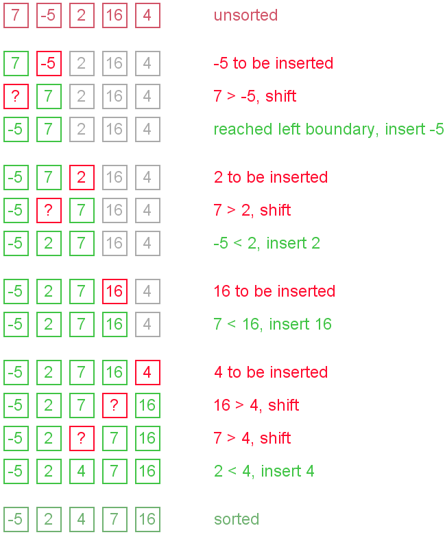
Let us see an example of insertion sort routine to make the idea of algorithm clearer.
Example. Sort {7, -5, 2, 16, 4} using insertion sort.
The ideas of insertion
The main operation of the algorithm is insertion. The task is to insert a value into the sorted part of the array. Let us see the variants of how we can do it.
"Sifting down" using swaps
The simplest way to insert next element into the sorted part is to sift it down, until it occupies correct position. Initially the element stays right after the sorted part. At each step algorithm compares the element with one before it and, if they stay in reversed order, swap them. Let us see an illustration.
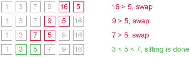
This approach writes sifted element to temporary position many times. Next implementation eliminates those unnecessary writes.
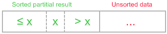
Shifting instead of swapping
We can modify previous algorithm, so it will write sifted element only to the final correct position. Let us see an illustration.
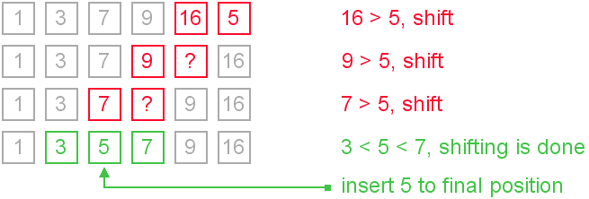
It is the most commonly used modification of the insertion sort.
Using binary search
It is reasonable to use binary search algorithm to find a proper place for insertion. This variant of the insertion sort is calledbinary insertion sort. After position for insertion is found, algorithm shifts the part of the array and inserts the element. This version has lower number of comparisons, but overall average complexity remains O(n2). From a practical point of view this improvement is not very important, because insertion sort is used on quite small data sets.
Complexity analysis
Insertion sort's overall complexity is O(n2) on average, regardless of the method of insertion. On the almost sorted arrays insertion sort shows better performance, up to O(n) in case of applying insertion sort to a sorted array. Number of writes is O(n2) on average, but number of comparisons may vary depending on the insertion algorithm. It is O(n2) when shifting or swapping methods are used and O(n log n) for binary insertion sort.
From the point of view of practical application, an average complexity of the insertion sort is not so important. As it was mentioned above, insertion sort is applied to quite small data sets (from 8 to 12 elements). Therefore, first of all, a "practical performance" should be considered. In practice insertion sort outperforms most of the quadratic sorting algorithms, like selection sort or bubble sort.
Insertion sort properties
- adaptive (performance adapts to the initial order of elements);
- stable (insertion sort retains relative order of the same elements);
- in-place (requires constant amount of additional space);
- online (new elements can be added during the sort).
Code snippets
We show the idea of insertion with shifts in Java implementation and the idea of insertion using python code snippet.
Java implementation
void insertionSort(int[] arr) {
int i,j,newValue;
for(i=1;i<arr.length;i++){
newValue = arr[i];
j=i;
while(j>0&&arr[j-1]>newValue){
arr[j] = arr[j-1];
j--;
}
arr[j] = newValue;
}
Python implementation
void insertionSort(L) {
for i in range(l,len(L)):
j = i
newValue = L[i]
while j > 0 and L[j - 1] >L[j]:
L[j] = L[j - 1]
j = j-1
}
L[j] = newValue
}
}
|
Binary search algorithm
Generally, to find a value in unsorted array, we should look through elements of an array one by one, until searched value is found. In case of searched value is absent from array, we go through all elements. In average, complexity of such an algorithm is proportional to the length of the array.
Situation changes significantly, when array is sorted. If we know it, random access capability can be utilized very efficientlyto find searched value quick. Cost of searching algorithm reduces to binary logarithm of the array length. For reference, log2(1 000 000) ≈ 20. It means, that in worst case, algorithm makes 20 steps to find a value in sorted array of a million elements or to say, that it doesn't present it the array.
Algorithm
Algorithm is quite simple. It can be done either recursively or iteratively:
- get the middle element;
- if the middle element equals to the searched value, the algorithm stops;
- otherwise, two cases are possible:
- searched value is less, than the middle element. In this case, go to the step 1 for the part of the array, before middle element.
- searched value is greater, than the middle element. In this case, go to the step 1 for the part of the array, after middle element.
Now we should define, when iterations should stop. First case is when searched element is found. Second one is when subarray has no elements. In this case, we can conclude, that searched value doesn't present in the array.
Examples
Example 1. Find 6 in {-1, 5, 6, 18, 19, 25, 46, 78, 102, 114}.
Step 1 (middle element is 19 > 6): -1 5 6 18 19 25 46 78 102 114
Step 2 (middle element is 5 < 6): -1 5 6 18 19 25 46 78 102 114
Step 3 (middle element is 6 == 6): -1 5 6 18 19 25 46 78 102 114
Example 2. Find 103 in {-1, 5, 6, 18, 19, 25, 46, 78, 102, 114}.
Step 1 (middle element is 19 < 103): -1 5 6 18 19 25 46 78 102 114
Step 2 (middle element is 78 < 103): -1 5 6 18 19 25 46 78 102 114
Step 3 (middle element is 102 < 103): -1 5 6 18 19 25 46 78 102 114
Step 4 (middle element is 114 > 103): -1 5 6 18 19 25 46 78 102 114
Step 5 (searched value is absent): -1 5 6 18 19 25 46 78 102 114
Complexity analysis
Huge advantage of this algorithm is that it's complexity depends on the array size logarithmically in worst case. In practice it means, that algorithm will do at most log2(n) iterations, which is a very small number even for big arrays. It can be proved very easily. Indeed, on every step the size of the searched part is reduced by half. Algorithm stops, when there are no elements to search in. Therefore, solving following inequality in whole numbers:
n / 2iterations > 0
resulting in
iterations <= log2(n).
It means, that binary search algorithm time complexity is O(log2(n)).
Code snippets.
You can see recursive solution for Java and iterative for python below.
Java
int binarySearch(int[] array, int value, int left, int right) {
if (left > right)
return -1;
int middle = left + (right-left) / 2;
if (array[middle] == value)
return middle;
if (array[middle] > value)
return binarySearch(array, value, left, middle - 1);
else
return binarySearch(array, value, middle + 1, right);
}
Python
def biSearch(L,e,first,last):
if last - first < 2: return L[first] == e or L[last] == e
mid = first + (last-first)/2
if L[mid] ==e: return True
if L[mid]> e :
return biSearch(L,e,first,mid-1)
return biSearch(L,e,mid+1,last)
|
Merge sort is an O(n log n) comparison-based sorting algorithm. Most implementations produce a stable sort, meaning that the implementation preserves the input order of equal elements in the sorted output. It is a divide and conquer algorithm. Merge sort was invented by John von Neumann in 1945. A detailed description and analysis of bottom-up mergesort appeared in a report byGoldstine and Neumann as early as 1948
divide and conquer algorithm: 1, split the problem into several subproblem of the same type. 2,solove independetly. 3 combine those solutions
Python Implement
def mergeSort(L):
if len(L) < 2 :
return L
middle = len(L)/2
left = mergeSort(L[:mddle])
right = mergeSort(L[middle:])
together = merge(left,right)
return together
Algorithm to merge sorted arrays
In the article we present an algorithm for merging two sorted arrays. One can learn how to operate with several arrays and master read/write indices. Also, the algorithm has certain applications in practice, for instance in merge sort.
Merge algorithm
Assume, that both arrays are sorted in ascending order and we want resulting array to maintain the same order. Algorithm to merge two arrays A[0..m-1] and B[0..n-1] into an array C[0..m+n-1] is as following:
- Introduce read-indices i, j to traverse arrays A and B, accordingly. Introduce write-index k to store position of the first free cell in the resulting array. By default i = j = k = 0.
- At each step: if both indices are in range (i < m and j < n), choose minimum of (A[i], B[j]) and write it toC[k]. Otherwise go to step 4.
- Increase k and index of the array, algorithm located minimal value at, by one. Repeat step 2.
- Copy the rest values from the array, which index is still in range, to the resulting array.
Enhancements
Algorithm could be enhanced in many ways. For instance, it is reasonable to check, if A[m - 1] < B[0] orB[n - 1] < A[0]. In any of those cases, there is no need to do more comparisons. Algorithm could just copy source arrays in the resulting one in the right order. More complicated enhancements may include searching for interleaving parts and run merge algorithm for them only. It could save up much time, when sizes of merged arrays differ in scores of times.
Complexity analysis
Merge algorithm's time complexity is O(n + m). Additionally, it requires O(n + m) additional space to store resulting array.
Code snippets
Java implementation
// size of C array must be equal or greater than
// sum of A and B arrays' sizes
public void merge(int[] A, int[] B, int[] C) {
int i,j,k ;
i = 0;
j=0;
k=0;
m = A.length;
n = B.length;
while(i < m && j < n){
if(A[i]<= B[j]){
C[k] = A[i];
i++;
}else{
C[k] = B[j];
j++;
}
k++;
while(i<m){
C[k] = A[i]
i++;
k++;
}
while(j<n){
C[k] = B[j]
j++;
k++;
}
Python implementation
def merege(left,right):
result = []
i,j = 0
while i< len(left) and j < len(right):
if left[i]<= right[j]:
result.append(left[i])
i = i + 1
else:
result.append(right[j])
j = j + 1
while i< len(left):
result.append(left[i])
i = i + 1
while j< len(right):
result.append(right[j])
j = j + 1
return result
MergSort:
import operator
def mergeSort(L, compare = operator.lt):
if len(L) < 2:
return L[:]
else:
middle = int(len(L)/2)
left = mergeSort(L[:middle], compare)
right= mergeSort(L[middle:], compare)
return merge(left, right, compare)
def merge(left, right, compare):
result = []
i, j = 0, 0
while i < len(left) and j < len(right):
if compare(left[i], right[j]):
result.append(left[i])
i += 1
else:
result.append(right[j])
j += 1
while i < len(left):
result.append(left[i])
i += 1
while j < len(right):
result.append(right[j])
j += 1
return result
|
Selection Sort
Selection sort is one of the O(n2) sorting algorithms, which makes it quite inefficient for sorting large data volumes. Selection sort is notable for its programming simplicity and it can over perform other sorts in certain situations (see complexity analysis for more details).
Algorithm
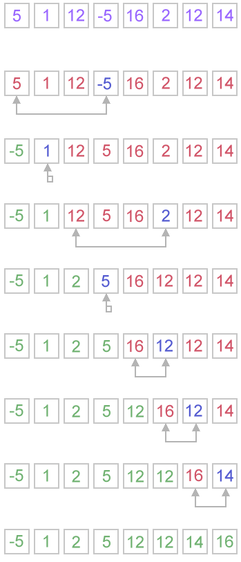
The idea of algorithm is quite simple. Array is imaginary divided into two parts - sorted one and unsorted one. At the beginning, sorted part is empty, while unsorted one contains whole array. At every step, algorithm finds minimal element in the unsorted part and adds it to the end of the sorted one. When unsorted part becomes empty, algorithmstops.
When algorithm sorts an array, it swaps first element of unsorted part with minimal element and then it is included to the sorted part. This implementation of selection sort in not stable. In case of linked list is sorted, and, instead of swaps, minimal element is linked to the unsorted part, selection sort is stable.
Let us see an example of sorting an array to make the idea of selection sort clearer.
Example. Sort {5, 1, 12, -5, 16, 2, 12, 14} using selection sort.
Complexity analysis
Selection sort stops, when unsorted part becomes empty. As we know, on every step number of unsorted elements decreased by one. Therefore, selection sort makes n steps (n is number of elements in array) of outer loop, before stop. Every step of outer loop requires finding minimum in unsorted part. Summing up, n + (n - 1) + (n - 2) + ... + 1, results in O(n2) number of comparisons. Number of swaps may vary from zero (in case of sorted array) to n - 1 (in case array was sorted in reversed order), which results in O(n) number of swaps. Overall algorithm complexity is O(n2).
Fact, that selection sort requires n - 1 number of swaps at most, makes it very efficient in situations, when write operation is significantly more expensive, than read operation.
Code snippets
Java
public void selectionSort(int[] arr) {
int i, j, minIndex, tmp;
int n = arr.length;
for (i = 0; i < n - 1; i++) {
minIndex = i;
for (j = i + 1; j < n; j++)
if (arr[j] < arr[minIndex])
minIndex = j;
if (minIndex != i) {
tmp = arr[i];
arr[i] = arr[minIndex];
arr[minIndex] = tmp;
}
}
}
Python
for i in range(len(L)-1): minIndex = i minValue = L[i] j = i + 1 while j< len(L): if minValue > L[j]: minIndex = j minValue = L[j] j += 1 if minIndex != i: temp = L[i] L[i] = L[minIndex] L[minIndex] = temp
|
Bubble Sort
Bubble sort is a simple and well-known sorting algorithm. It is used in practice once in a blue moon and its main application is to make an introduction to the sorting algorithms. Bubble sort belongs to O(n2) sorting algorithms, which makes it quite inefficient for sorting large data volumes. Bubble sort is stable and adaptive.
Algorithm
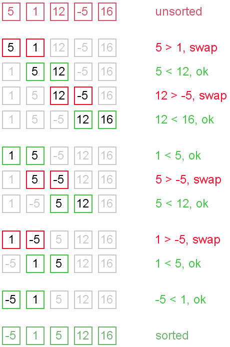
- Compare each pair of adjacent elements from the beginning of an array and, if they are in reversed order, swap them.
- If at least one swap has been done, repeat step 1.
You can imagine that on every step big bubbles float to the surface and stay there. At the step, when no bubble moves, sorting stops. Let us see an example of sorting an array to make the idea of bubble sort clearer.
Example. Sort {5, 1, 12, -5, 16} using bubble sort.
Complexity analysis
Average and worst case complexity of bubble sort is O(n2). Also, it makes O(n2) swaps in the worst case. Bubble sort is adaptive. It means that for almost sorted array it gives O(n) estimation. Avoid implementations, which don't check if the array is already sorted on every step (any swaps made). This check is necessary, in order to preserve adaptive property.
Turtles and rabbits
One more problem of bubble sort is that its running time badly depends on the initial order of the elements. Big elements (rabbits) go up fast, while small ones (turtles) go down very slow. This problem is solved in the Cocktail sort.
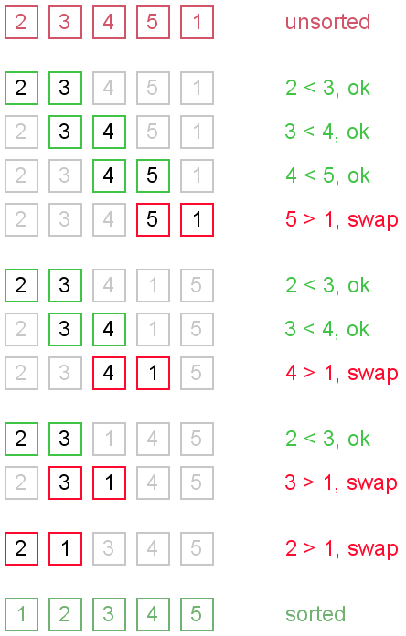
Turtle example. Thought, array {2, 3, 4, 5, 1} is almost sorted, it takes O(n2) iterations to sort an array. Element {1} is a turtle.
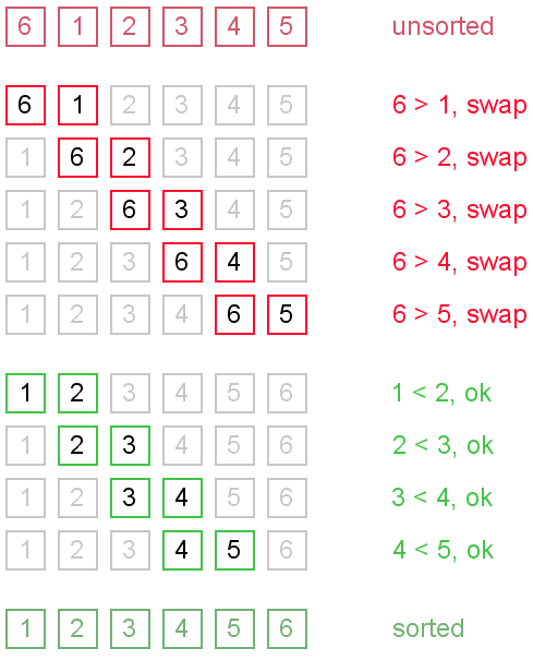
Rabbit example. Array {6, 1, 2, 3, 4, 5} is almost sorted too, but it takes O(n) iterations to sort it. Element {6} is a rabbit. This example demonstrates adaptive property of the bubble sort.
Code snippets
There are several ways to implement the bubble sort. Notice, that "swaps" check is absolutely necessary, in order to preserve adaptive property.
Java
public void bubbleSort(int[] arr) {
boolean swapped = true;
int j = 0;
int tmp;
while (swapped) {
swapped = false;
j++;
for (int i = 0; i < arr.length - j; i++) {
if (arr[i] > arr[i + 1]) {
tmp = arr[i];
arr[i] = arr[i + 1];
arr[i + 1] = tmp;
swapped = true;
}
}
}
}
Python
def bubbleSort(L) :
swapped = True;
while swapped:
swapped = False
for i in range(len(L)-1):
if L[i]>L[i+1]:
temp = L[i]
L[i] = L[i+1]
L[i+1] = temp
swapped = True
|
摘要: 關(guān)于二分查找的原理互聯(lián)網(wǎng)上相關(guān)的文章很多,我就不重復(fù)了,但網(wǎng)絡(luò)的文章大部分講述的二分查找都是其中的核心部分,是不完備的和效率其實(shí)還可以提高,如取中間索引使用開始索引加上末尾索引的和除以2,這種做法在數(shù)字的長度超過整型的范圍的時候就會拋出異常,下面是我的代碼,其中可能有些地方?jīng)]考慮到或有什么不足 閱讀全文
|